Have you ever typed a number with one or more leading zeros, like 00123 and watched as Excel drops the leading zeros as soon as you press Enter.
Frustrating, isn’t it!
So how do you fix it?
There are 2 methods. One is better than the other for a quick set up and easy maintenance. There is also a third method which combines elements from each of the first two.
Method 1: Format the cells as text
1. Before you enter any data, select the cells where the data is to be entered.
2. Press CTRL 1. This is a keyboard shortcut to display the Format Cells dialog.
3. On the Number tab, choose the TEXT category.
4. Close the dialog.
Now, when you enter your data with leading zeros, the leading zeros remain and do not disappear when you press Enter.
A couple of things to watch out for:
1. Text is left-aligned by default so you may need to re-align the data.
2. If your data has already been entered (or downloaded), switching to a text format will not fix the data - there is a partial fix for this which is outlined in Method 3.
Method 2: Use custom formatting
1. Select the cell range where the data will be entered (or has already been entered).
2. Press CTRL 1 to display the Format Cells dialog.
3. In the Number tab, choose the CUSTOM category.
4. Custom formatting works with a system of place holders. For numbers, the primary place holders are:
5. If you have a 5 digit product code, enter 00000 into the TYPE box. This will convert 123 to 00123, 1 to 00001 etc.
6. If you have a phone number with a 4-digit area code followed by 2 sets of 4 digits, enter (0000) 000-000 into the TYPE box. This will convert 0123456789 to (0123) 456-789.
7. Close the dialog.
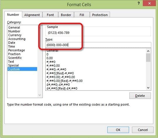
Figure 01: Create a custom format
The new custom format will now be applied.
Phone numbers will now have the punctuation and spacing. For example, enter 0123456789 into a custom-formatted phone number cell (see above) and press Enter. It will automatically reformat to (0123) 456–789.
Numbers that previously dropped the leading zeros will now display the leading zeros. For example, enter 123 into a custom-formatted number cell (see above) and press Enter. The leading zero will be added automatically to display 00123.
Method 3: Expert Tip - Combine methods 1 and 2
If you import data into Excel that was exported from another program or website, the data is often formatted entirely as text.
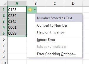
Figure 02: Numbers stored as text
You can click the smart icon (see above), then choose Convert To Number but you still don’t have the leading zeroes!
An easy way to convert a lot of ‘text’ numbers to ‘numeric’ numbers (if that makes sense) and add leading zeroes is to follow this process (assume the ‘text’ numbers are in column A):
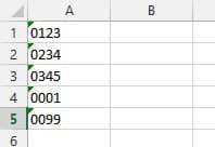
Figure 03: Numbers start in text format
1. Insert a blank column, if necessary.
2. In cell B1 type =A1*1 and press Enter. The result is the same number but in numeric format (notice that it is right-aligned).
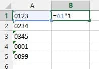
Figure 04: Formula that converts 'text' number to 'numeric' number
3. Copy the formula down.
4. Select column B and assign the custom format to add the leading zeros as described above.
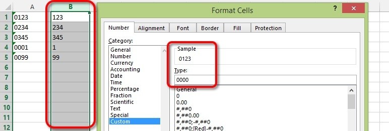
Figure 05: Select the entire column and set a custom format
5. With column B still selected, COPY the data then PASTE SPECIAL as VALUES (using the right-click menu) to column B to overwrite the values, or PASTE SPECIAL directly over the original ‘text’ numbers in column A if your prefer.

Figure 06: Select the column of data, COPY, then PASTE SPECIAL the VALUES over the same cells
6. Delete column B as it is now redundant.
I hope that gets you out of a fix.
What do you think?
Watch the video (over the shoulder demo)
To see this technique demonstrated with additional examples, check out this Leading Zeroes video.

What next?
I hope you found plenty of value in this post. I'd love to hear your biggest takeaway in the comments below together with any questions you may have.
Have a fantastic day.


About the author
Jason Morrell
Jason Morrell is a professional trainer, consultant and course creator who lives on the glorious Gold Coast in Queensland, Australia.
He helps people of all levels unleash and leverage the power contained within Microsoft Office by delivering training, troubleshooting services and taking on client projects. He loves to simplify tricky concepts and provide helpful, proven, actionable advice that can be implemented for quick results.
Purely for amusement he sometimes talks about himself in the third person.
SHARE

