
In the previous post, you discovered how easy it is to calculate a total using the AUTOSUM button. In this post I expand on that and discuss 4 other basic formula functions that are also useful and easy to use - AVERAGE, MAX, MIN and COUNT.
1. Our example data
Let’s take a look at a simple table showing the number of kilometres driven each month.
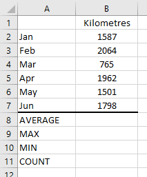
Figure 01: Kilometre distance table
All 4 functions - AVERAGE MAX, MIN and COUNT are actually found on the AUTOSUM button, but are only displayed when you click the little drop-down arrow, as you'll see in a moment.
I’m going to show you how to calculate the AVERAGE monthly distance, the LONGEST distance, the SHORTEST distance and HOW MANY monthly figures are in the list.
With each function, just like with AUTOSUM, you can start by selecting the blank answer cell
… OR the 6 cells containing the figures
… OR the 6 cells containing the figures AND the blank answer cell.
2. The AVERAGE Function
To calculate the AVERAGE monthly distance:
1. Select cell B8.
2. Click the drop-down arrow on the AUTOSUM button.
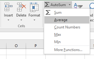
Figure 02: Choose the AVERAGE function from the AutoSum drop-down list
3. Choose AVERAGE.
4. Press ENTER to confirm the cell range.
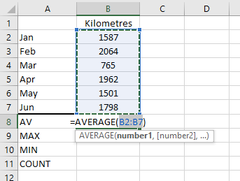
Figure 03: The AVERAGE Function
3. The MAX Function
To find the LONGEST distance:
1. Select cell B9.
2. Click the drop-down arrow on the AUTOSUM button.
3. Choose MAX.
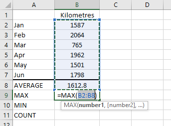
Figure 04: The MAX Function
At this point, the range that Excel has identified is too large so using the mouse, select cells B2:B7.
4. Press ENTER to confirm the cell range.
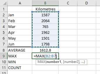
Figure 04a: Fix the cell range for the MAX function
MAX can be used whenever you need to find the figure that is the LONGEST, TALLEST, LARGEST, MOST etc.
4. The MIN Function
To find the SHORTEST distance:
1. Select cell B10.
2. Click the drop-down arrow on the AUTOSUM button.
3. Choose MIN.
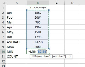
Figure 05: The MIN Function
At this point, the range that Excel has identified is too large so using the mouse, select cells B2:B7.
4. Press ENTER to confirm the cell range.
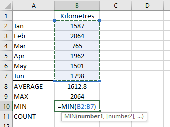
Figure 05a: Fix the cell range for the MIN function
MIN can be used whenever you need to find the figure that is the SHORTEST, LOWEST, SMALLEST, LEAST etc.
5. The COUNT Function
To find HOW MANY figures in the list:
1. Select cell B11.
2. Click the drop-down arrow on the AUTOSUM button.
3. Choose COUNT NUMBERS.
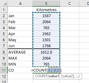
Figure 06: The COUNT Function
At this point, the range that Excel has identified is too large so using the mouse, select cells B2:B7.
4. Press ENTER to confirm the cell range.
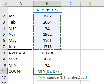
Figure 06a: Fix the cell range for the COUNT function
Use COUNT whenever you need an answer to a HOW MANY type question.
Because COUNT NUMBERS only counts how many cells contain numbers, (hence the name) if a number is deleted or overwritten with text and/or symbols, these cells will be ignored and the count will decrease.
6. Excel Auto-Stats
Whenever two or more cells are selected, a number of stats are automatically displayed on the status bar.
![[4 Basic Functions] AVERAGE etc Image 7 - Auto Stats on the Status Bar AVERAGE etc Image 7 - Auto Stats on the Status Bar](https://d1pzfp4ixszkr4.cloudfront.net/img/2016/12/01100134/Image-7-Auto-Stats.jpg)
Figure 07: Auto Stats on the Status Bar
The stats available are
As you can see, they tie in closely with the functions covered above. The difference between COUNT and COUNT NUMBERS is that the first will count how many cells are populated while the second only counts the cells containing numbers. Both are useful.
To show more or less of these stats:
1. Right-click anywhere on the status bar
2. About two thirds of the way down, tick the stats you wish to see on the status bar.
![[4 Basic Functions] AVERAGE etc Image 8 - Selecting which Auto Stats appear on the Status Bar AVERAGE etc Image 8 - Selecting which Auto Stats appear on the Status Bar](https://d1pzfp4ixszkr4.cloudfront.net/img/2016/12/01100134/Image-8-Auto-Stat-Options.jpg)
Figure 8: Selecting which Auto Stats appear on the Status Bar
Don’t forget, once you have made your changes, you must first select two or more cells to see the stats appear on the status bar.
7. Watch the video (over the shoulder demo)

8. What Next?
In the next and final post in this mini-series, I discuss the importance of the ‘Order of Operations’. It resurrects some old math skills from the archives of your brain but you need to know and master this before you go any further with Excel.
Even seasoned Excel pros sometimes get this wrong, and there have been stories of companies losing millions of dollars due to simple mathematical errors with formulas in Excel. Make sure you don’t make the same mistakes.
See you there.
I hope you found plenty of value in this post. I'd love to hear your biggest takeaway in the comments below together with any questions you may have.
Have a fantastic day.


About the author
Jason Morrell
Jason Morrell is a professional trainer, consultant and course creator who lives on the glorious Gold Coast in Queensland, Australia.
He helps people of all levels unleash and leverage the power contained within Microsoft Office by delivering training, troubleshooting services and taking on client projects. He loves to simplify tricky concepts and provide helpful, proven, actionable advice that can be implemented for quick results.
Purely for amusement he sometimes talks about himself in the third person.
SHARE

