Drop-down lists in Excel not only look cool but they limit the options available which reduces errors during the input process. And they're not as hard as you might think.
That said, if you don't set them up right, they become a nuisance to maintain. This post walks you through the process to set them up in the best, easiest and most flexible way.
1. Why is a drop-down list useful?
Using a drop down list in Excel serves a number of useful functions:

Figure 01: Using a drop-down list has many advantages
2. How to create a dropdown list in Excel
You can create a drop down list in 2 entirely different ways. The first way is to create a combo box using the form controls on the Developer tab. That method is not the focus of this post. The second way, discussed below, is to use the Data Validation feature.
Step 1: Create Your List
The first thing you need is a list. Many people dedicate a worksheet to any lists they use. This worksheet can be hidden to keep it from prying eyes, but you know it’s there so you can unhide it and maintain it in the future.
Let’s say you create a list of 5 items in cells A1 to A5.
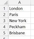
Figure 02: Type your list items
An optional, but useful step is to name the range.
1. Select cells A1:A5.
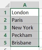
Figure 03: Select the cell range containing your list
2. Click in the name box (to the left of the formula bar).

Figure 04: Click in the Name Box
3. Overtype the current cell reference (A1) with a name, e.g. Locations.
Figure 05: Click in the Name Box
If you ever want to name a cell or cell range using 2 or more words, just separate them with an underscore (_), e.g. Customer_Locations or butt the words up against each other, e.g. CustomerLocations.
One handy benefit of naming cells is that you can use the name in formulas wherever you are in the spreadsheet, so you don’t have to navigate backwards and forwards to find the cells that contain the list.
Step 2: Add a drop down list to cell(s)
Next you need to add the drop down lists to your cells.
1. Select the cell(s) where the drop down list will appear.
 Figure 06: Select the cell(s) that will have the drop-down lists
Figure 06: Select the cell(s) that will have the drop-down lists
2. Click the Data tab.
3. Click the Data Validation icon (i.e. not the drop-down component) to display the Data Validation dialog box.
Figure 07: Click the top half of the Data Validation icon
4. In the Settings tab, in the Allow box, choose List.
5. Position the cursor in the Source box.
6. Press F3 to display a list of all named cells or cell ranges.
7. Choose your named range from the list. The Source box will now say: =YourListName.
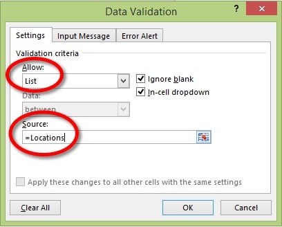
Figure 08: The Settings tab
8. Click the Input Message tab.
9. Untick the box labelled ‘Show input message when cell is selected’ as most people already know what to do with a drop down arrow and a drop down list.
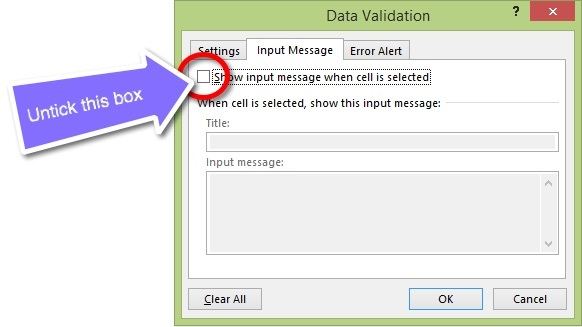
Figure 09: The Input Message tab
10. If you want to ensure that only an item from your list is selected, click the Error Alert tab and complete the title and message information to display a more user-friendly message than the default that Microsoft give you.
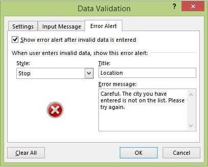
Figure 10: The Error Alert tab
11. [Optional step] Change the Style option from Stop (fix the error or cancel) to Warning (Whoops! Can’t find that entry – wanna keep it – Yes or No) or Information (Whoops! I don’t recognise that – OK or cancel).
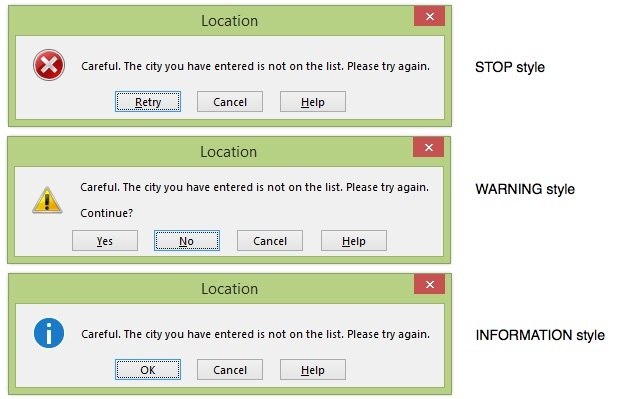
Figure 11: The 3 different Error Alert styles
11. Close the dialog box.
Step 3: Test it
The setup is now complete, so let’s see how the drop down list looks.
1. Click any cell that has the data validation. A drop down arrow will appear.
2. Click the drop down arrow and the drop down list is displayed.
3. Select the item from the list.

Figure 12: Using a drop-down list has many advantages
4. Type in one of the entries, correctly. It will be accepted, no problems.
5. Mis-type an entry. The error message will be displayed.
3. Re-using the same drop down lists in other cells
What if you need to apply the same validation to other cells?
1. Select the last cell that has validation on it.
2. Use the autofill handle (the block on the bottom-right corner of the cell) to copy the validation downwards, thereby extending the range of cells using the drop down list.
3. You can also Copy and Paste Special the Validation directly to other cells.
As you can see, it’s pretty neat.
4. Maintaining your list
At some point you’ll probably want to extend the list, remove some items or change some of the entries on the list. Let’s re-visit the list.
Any entries that are edited are effective immediately, so all drop down lists will now use the new values.
Let’s add a couple of new items to the list.
To check that the new items are included:
1. Click the Formulas tab.
2. Select the Name Manager icon to display the Name Manager dialog.
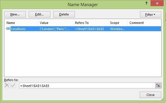
Figure 13: The Name Manager dialog
3. Select your list name and check that the cell range is correct. If it isn’t you can very carefully edit the current range in the Refers To box or reselect the new larger range directly on the sheet.
4. Close the dialog box.
Job done.
5. Applying validation to existing data
One last thing. If you have been handed a spreadsheet, you can apply validation to existing data. The data may be good, bad or mixed. There’s a great tool to highlight the bad data so it can be rectified.
1. Set up the drop down lists using the data validation tool as described above.
2. Click the drop-down arrow on the Data Validation tool.
3. Select Circle Invalid Data.
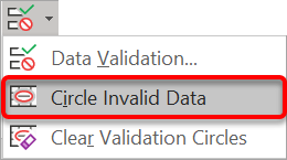
Figure 14: Circling invalid data
All entries that don’t match one of the items on your list will be circled. Can’t miss it!

Figure 15: Invalid data can be circled in red so that you can quickly see what needs to be fixed
6. Watch the video (over the shoulder demo)

7. What next?
So there you have it.
If you don’t currently use drop down lists, try creating one (or several) today. You can literally be up and running within 60 seconds.
I hope you found plenty of value in this post. I'd love to hear your biggest takeaway in the comments below together with any questions you may have.
Have a fantastic day.


About the author
Jason Morrell
Jason Morrell is a professional trainer, consultant and course creator who lives on the glorious Gold Coast in Queensland, Australia.
He helps people of all levels unleash and leverage the power contained within Microsoft Office by delivering training, troubleshooting services and taking on client projects. He loves to simplify tricky concepts and provide helpful, proven, actionable advice that can be implemented for quick results.
Purely for amusement he sometimes talks about himself in the third person.
SHARE


hello, i really enjoyed this and it will be very helpful as i navigate through excel. i do have a pretty direct question that i am struggling to find help with.
i have a drop down list in column A2-A13. this list is from a seperate tab. each item in the list is linked to a formula. so when i pick the item from the drop down, it pulls the formula. the answer provided goes into column C.
Here is the tricky part. all the formulas are linked to the number you input in B2 on the main tab. “so if i pick countersink in cell A2 from the list, the formula attached is main1B2*20+15. this works great to provide an answer in C2, but when i pick something from the list in A3-A13, it still pulls the formula but still links it to the number inputted in B2 instead of finding the corresponding “B column” that matches the item picked in the “A” column.
i am struggling just trying to explain this so searching google has been frustrating. i know this is a long shot to get a reply but figured what the hell.
Hi Eric. I don’t quite get all that you’re saying but assuming you have 2 sheets called Main and List, try this approach.
On the List sheet:
1. In column A you have the items that appear in your dropdown list, let’s say Item 1 thru Item 12.
2. In column B you have the corresponding values that you want to use in your formula.
3. Format as Table.
4. Name the cells in column A (let’s say ‘Items’, for use in your drop-down validation source).
5. Name all the cells used in columns A and B (let’s say ‘ItemTable’, for use in your formula – see below).
On the Main sheet:
1. Set up the validation in cells A2:A13, using =Items in your source box.
2. In cell B2 write this formula: =VLOOKUP(A2, ItemTable, 2, FALSE)*20+15
3. Copy/fill cell B2 down to B13.
I’m not aware of your whole setup but you should be able to adapt and work it out from the information above. Let me know how you go.