Validating data is important. Whether you do it at the point when data is entered or you want to check a finished workbook, the data validation process is a good investment of your time.
Good data IN means accurate data OUT. In other words, your reports will reflect the true results.
In this post you'll discover what kinds of data can be validated, how to set up and manage the data validation settings and see some examples being constructed.
1. Why does data need to be validated?
Many problems in Excel can be traced back to bad data, which includes numerical data that is out of range, incorrect dates or typos in the text.
Data Validation allows you to
When you identify invalid data at the front-end and address it, the results and reports produced on the back end are more accurate.
When data validation is applied, it ensures that you are working with ‘clean’ data and to some degree gets you towards the holy grail of creating an IDIOT PROOF spreadsheet! (Famous Last Words)
2. What type of data can be validated?
3. How to apply Data Validation
To create validation rules:
1. Click the cell or cell range that you wish to validate.
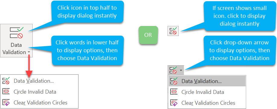
2. Click the Data Validation icon on the Data ribbon. If your screen displays a large icon, the top half will display the dialog directly, but the lower half will display a sub-menu where you need to click Data Validation to open the dialog.
3. In the dialog, three tabs are presented. Settings, Input Message and Error Alert tab.
4. Set the Validation rules (Settings tab)
![[E2] 07 - 02 setting the rules Setting the rules (settings tab)](http://officemastery.com/wp-content/uploads/2020/03/E2-07-02-setting-the-rules.png)
This tab is used to specify what valid data looks like.
1. Choose an option from the Allow box.
2. Complete the boxes that are then displayed (each type has different options. Following are some examples.
5. User Instructions (Input Message tab)
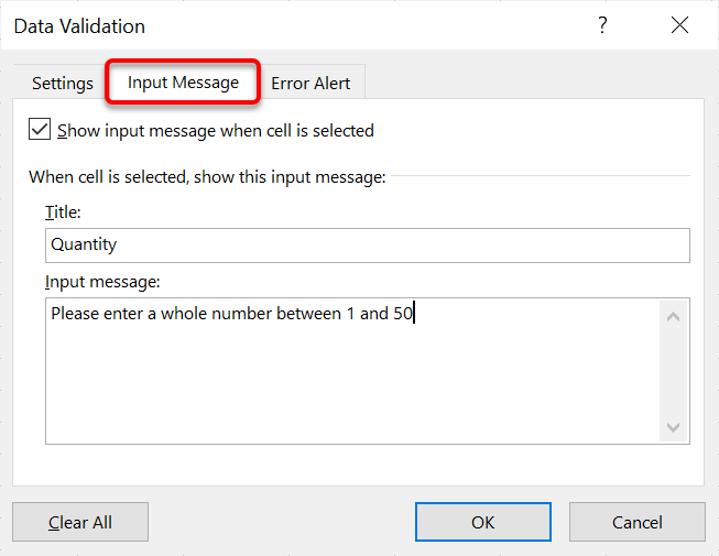
This tab is used to give the user instructions or guidelines about what data to enter in the cell.
1. Enter a title and an instruction.
2. The input message is optional. To switch it off, clear the Show input message when cell is selected box.
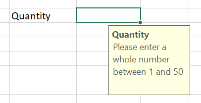
When the user clicks the cell that contains data validation, a screen tip is displayed as a guide.
6. Alert the user of errors (Error Alert tab)
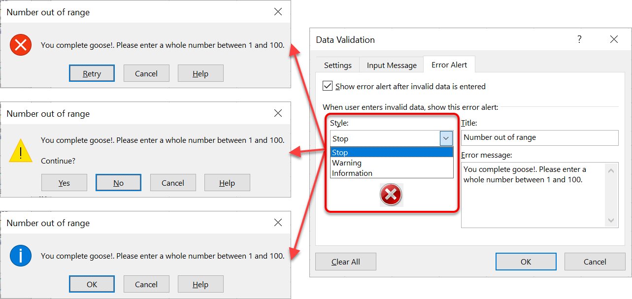
This tab is used to display an alert message indicating that the data is invalid.
1. Enter a title and an error message to highlight the problem.
2. Set a Style. The style can be changed to be strict or lenient.
Or untick Show error alert after invalid data is entered to switch off the alert message.
7. Highlight invalid data on your worksheet
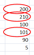
Whether you deliberately let invalid data through the net, or you have just set up validation on an existing worksheet, you can instantly flag all invalid data.
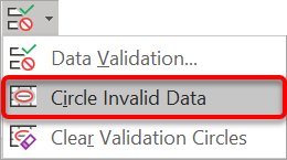
1. Click the drop-down arrow on the Data Validation icon (on the Data ribbon).
2. Choose Circle Invalid Data.
3. To clear the circles, click the Data Validation button and choose Clear Validation Circles
8. Highlight all cells with validation rules
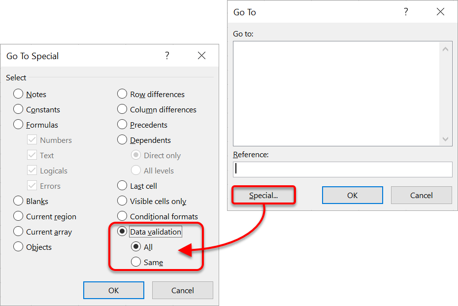
To locate cells that have active validation rules:
1. Press F5 or Ctrl G, then click Special... .
Or select the Home ribbon | Find & Select | Go To Special
2. Click the Data Validation option button (bottom-right).
3. Click All to find every cell with validation or Same to fond those cells with matching validation.
4. Click Ok
9. Ex01: Whole number > 100
In the Data Validation dialog, choose Whole Number | Greater than | 100
10. Ex02: Decimal Number <= 123.45
In the Data Validation dialog, choose Decimal | Less than or equal to| 123.45
11. Ex03: Date is in date range
In the Data Validation dialog, choose Date | Between | Start date and End date
12. Ex04: Text length is <= 15 characters
In the Data Validation dialog, choose Text length | Less than or equal to | 15
13. Ex05: Drop-down lists
Drop-down lists are one of the most effective ways to ensure you get valid data. Just pick from the list.
First you must set up your list.
1. Type or paste the items you wish to present in your drop-down list.
2. Select the cells and name the cell range (remember, no spaces, but underscores are allowed).
3. Format the table (Home ribbon | Format as Table). This makes future maintenance easy because when you add, remove or change items in your list, the table expands or shrinks automatically, and the changes are reflected immediately on your drop-down list.
Then create your drop-down list.
1. Select the cell(s) in which you wish to create a drop-down list.
2. Click the Data tab.
3. Click the Data Validation icon on the Data ribbon
4. In the Data Validation dialog, click the Settings tab.
5. In the Allow box, choose List.
6. Position the cursor in the Source box.
7. Press F3 to display a list of all named cells or cell ranges (if you named the range).
8. Choose your named range from the list. The Source box will now say, =<YourListName>.
9. Populate the Input Message and Error Alert tabs as necessary.
10. Close the dialog box.
Once the setup is complete, always test it, then propagate.
1. Click the drop-down arrow on the cell to display the drop-down list.
2. Select an item from the list. You already know it’s valid.
3. Overtype the contents of the cell with a valid list option. No problems.
4. Deliberately mis-type something in the cell. That’s when the error message is displayed.
5. Once you know it works, you can autofill the entire cell down or just the validation component using Paste Special è Validation.
Then’ it’s just a case of maintaining the list. Here’s some pointers.
14. Key Takeaways
I hope you found plenty of value in this post. I'd love to hear your biggest takeaway in the comments below together with any questions you may have.
Have a fantastic day.


About the author
Jason Morrell
Jason Morrell is a professional trainer, consultant and course creator who lives on the glorious Gold Coast in Queensland, Australia.
He helps people of all levels unleash and leverage the power contained within Microsoft Office by delivering training, troubleshooting services and taking on client projects. He loves to simplify tricky concepts and provide helpful, proven, actionable advice that can be implemented for quick results.
Purely for amusement he sometimes talks about himself in the third person.
SHARE

