In this post you'll discover an array of wonderful tools to format a spreadsheet and make it look fantastic.
If you're reading this, then I'm going to assume that you have already entered your data and written all the formulas you need.
If you haven't, then return to your spreadsheet and finish the data stage. Only then should you start formatting otherwise you'll be faffing around, chopping and changing and fiddling. And it will take 10 times as long. Trust me.
1. Quick number formatting
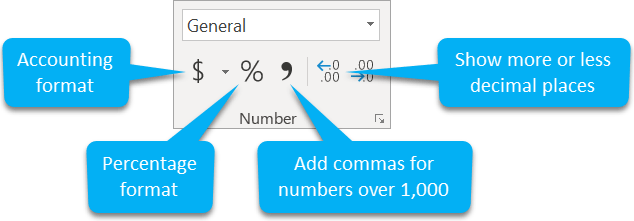
On the Home ribbon, front and centre, you’ll find the Number group with 5 useful tools for quick number formatting and a drop-down menu with options for other types of content like dates, accounting etc.
2. The Format Cells dialog
A cell may be formatted in a number of ways. From simple number formatting (like decimal places) to content styling, alignment, positioning, text control, borders and shading.
The control centre for anything related to cell formatting is the Format Cells dialog.
1. Click on the cell or cell range to be formatted.
2. Select the Home tab.
3. Click the launcher (pictured right) In the Number group
… or press Ctrl 1
… or right-click and choose Format Cells from the context menu.
The Format Cells dialog is now displayed.
3. How to format a number in Excel
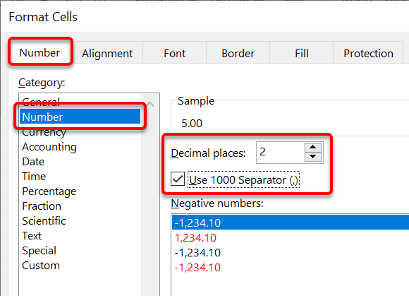
To control how a number is displayed (decimal places, 1,000 separator etc.):
1. Display the Format Cells dialog
2. Select the Number tab.
3. Select Number from the Category list.
4. Choose how many decimal places the number should have.
5. Decide whether to use a 1000 separator for numbers like 1,000 or 1,000,000.
6. Click OK
4. How to format a date in Excel
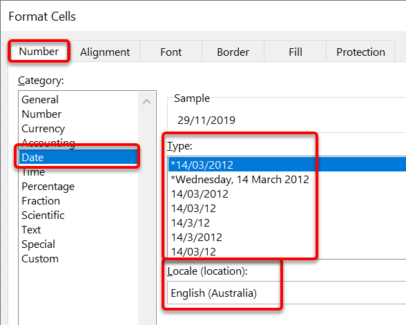
To change the way a date looks:
1. Display the Format Cells dialog
2. Select the Number tab.
3. Select Date from the Category list.
4. Ensure your locale (country or region) is set correctly.
5. Choose a date format from the Type list.
6. Click OK
5. How to rotate cell content
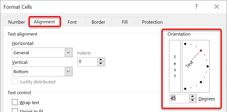
To angle text at 30, 45 or 90 degrees (or any angle for that matter):
1. Display the Format Cells dialog
2. Select the Alignment tab.
3. Drag the red diamond in the Orientation box to any position on the semi-circle (or click directly on the circle or type the degree figure in the box)
4. Click OK
6. How to position cell content in Excel
METHOD 1: Format Cells dialog
To set the horizontal and vertical positioning of cell content:
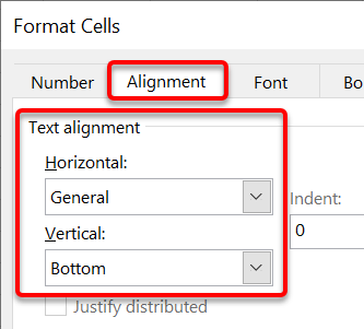
1. Display the Format Cells dialog
2. Select the Alignment tab.
3. Click the drop-down arrow on the Horizontal box and choose Left, Center,or Right.
4. Click the drop-down arrow on the Vertical box and choose Top, Middle or Bottom.
5. Click OK
METHOD 1: the Home ribbon
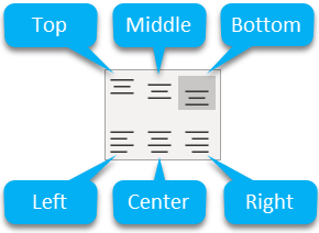
1. Select the HOME tab, if necessary.
2. Click any of the alignment icons in the Alignment group to set the horizontal and vertical alignment.
7. How to make cell content fit better
Sometimes text just doesn’t fit. There are two fantastic tools to handle this problem automatically.
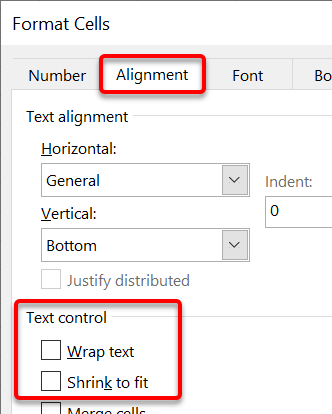
1. Display the Format Cells dialog
2. Select the Alignment tab.
3. Select Wrap Text to wrap text automatically to a new line if it is too wide (like the end of a line in a Word doc).
4. Or select Shrink to Fit to reduce the size of text to make it fit on one line using the current column width.
5. Click OK
In the Alignment group on the Font ribbon there is a button you can use. However, there is no Shrink to Fit button.
8. How to merge cells
For simple spreadsheets, it’s okay to merge cells. When spreadsheets become more complex, merging cells can create lots of problems. This is discussed (along with a remedy and alternative approach) in a higher-level course.
To merge two or more cells into one big cell:
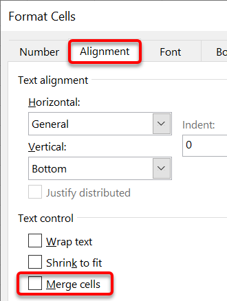
1. Select all the cells to be merged.
2. Display the Format Cells dialog
3. Select the Alignment tab.
4. Select Merge Cells.
5. Click OK
Microsoft realised that many people were merging cells then centring the content, so, they gave us a Merge & Center button on the Home ribbon to do just that.
9. Special formatting like strikethrough & superscript
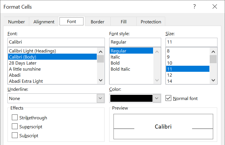
To set the font attributes that are not on the Home ribbon:
1. Display the Format Cells dialog
2. Select the Font tab.
3. Select a font, style, size and colour.
4. Choose an underline style by selecting from the drop-down list.
5. The Strikethrough will draw a line through the cell contents, like this.
6. Superscripted text is used for things like 32 and 13th.
7. Subscripted text is used for things like H2O.
8. Click OK
10. Drawing cell borders
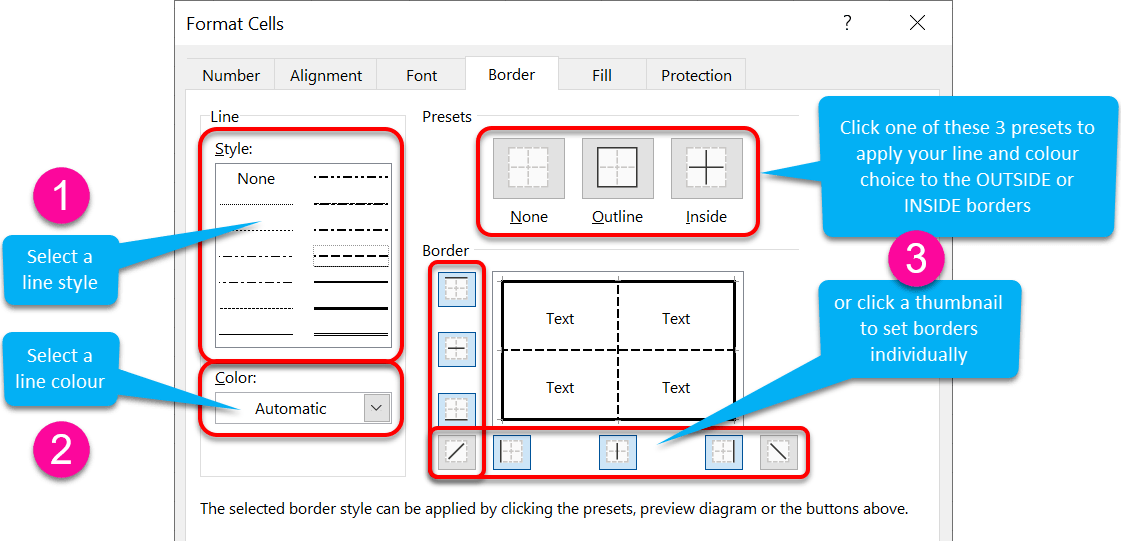
To draw printable borders:
1. Select the cells you wish to apply borders to.
2. Display the Format Cells dialog and select the Borders tab.
3. Select a line style.
4. Select a line colour.
5. Use one of the following techniques:
6. Click OK
11. Adding colour to cells in Excel
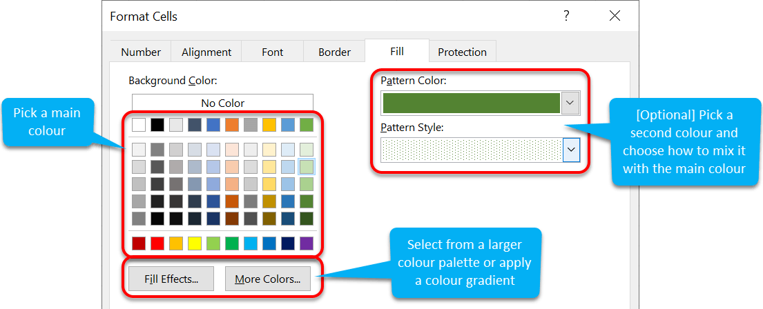
To add some colour and interest to your selected cells:
1. Display the Format Cells dialog
2. Select the Fill tab.
3. Select a colour from the colour palette.
4. To break up a colour, pick a pattern and pattern colour from the Pattern drop-down palette.
5. Click OK
12. two ways to use Format Painter
There is a beautiful little tool on the Home ribbon called Format Painter which allows you to copy the formatting from one cell or cell range to another.
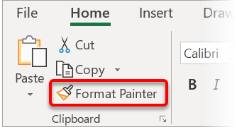
1. Select the cell or range of cells with the source formatting.
2. Click the Home tab, if necessary.
3. To copy the formatting once:
The formatting is copied, and the Painter is switched off.
4. To copy the formatting as many times as you want:
The formatting is copied, but the Painter remains on, so you can continue to apply the same formatting to additional cells or cell ranges.
5. To switch off the Format Painter, click the icon again or hit Esc (Escape).
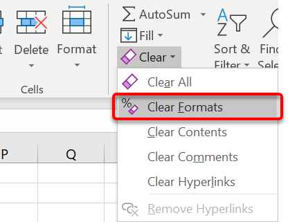
13. How to reset all cell formatting
To clear the formatting from a cell or cell range:
14. Using the Format-as-Table tool
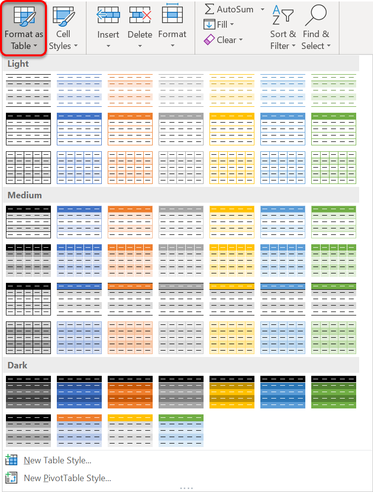
Excel provides many pre-set designs that you can use for your tables of data.
1. Click any cell in your data range.
2. Select the Home ribbon, if necessary.
3. Click the Format as Table button in the Styles group. A gallery is presented.
4. Choose a format design from the gallery (see next page).
5. Confirm whether your table already has headers, or you want Excel to create some for you.
15. Format a spreadsheet: Key takeaways
I hope you found plenty of value in this post. I'd love to hear your biggest takeaway in the comments below together with any questions you may have.
Have a fantastic day.


About the author
Jason Morrell
Jason Morrell is a professional trainer, consultant and course creator who lives on the glorious Gold Coast in Queensland, Australia.
He helps people of all levels unleash and leverage the power contained within Microsoft Office by delivering training, troubleshooting services and taking on client projects. He loves to simplify tricky concepts and provide helpful, proven, actionable advice that can be implemented for quick results.
Purely for amusement he sometimes talks about himself in the third person.
SHARE

