In this post you'll discover why naming cells or call ranges in Excel is so powerful. It adds a whole new level to your formulas and makes them easier to read and easier to maintain. There are lots of other reasons too.
You will see 2 methods to name cells and manage them. You can even apply your new cell names to existing formulas.
There's plenty to cover. Let's dive in.
1. Why should you name cells?
You can assign a name to a cell or a cell range. This introduces a number of benefits:
2. Naming cells using the Name box
The Name Box is located to the left of the formula bar and above the column labels. It displays the currently selected cell or the first cell of a cell range.
To name the cell or cell range:
1. Select the cell(s) to be named.
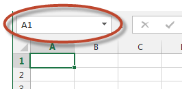
2. Click in the middle of the Name Box, not the drop-down arrow. The cell reference will now be highlighted.
3. Overtype the cell reference with a name. Spaces are not allowed but underscores ( _ ) are.
4. Press Enter to register the name. If you forget to press Enter, the name will not be registered, and you won’t be able to use it.
3. Naming cells using the Name Manager
To name a cell using the Name Manager:
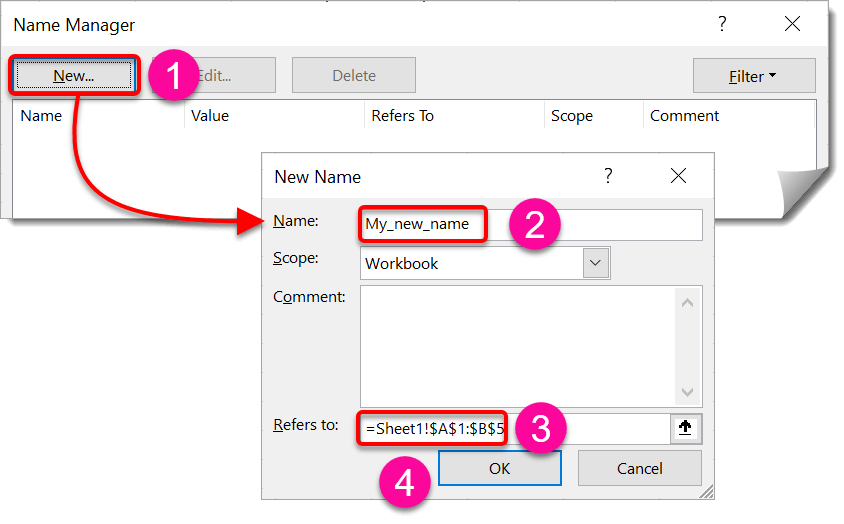
1. Click the Name Manager icon on the Formulas ribbon
The keyboard shortcut to display the Name Manager is Ctrl F3.
In the Name Manager dialog, all existing named cells or ranges are listed together with their current values and what cell or cell range the name refers to.
2. Click New.
3. In the New Name dialog, type a name (remember, no spaces but underscores are allowed).
4. Place the cursor in the Refers to box, then using the mouse, select the cell(s) to be named.
5. Add a comment if you want. Comments are useful in reminding you what the named cell(s) are used for and where they fit in the big picture.
6. Click Ok to create the Name.
4. How to create a constant
Named cell can be used as constants.
Constants are values that will never change such as the number of days in a year or mathematical PI.
To create a constant:
1. Click the Name Manager icon on the Formulas ribbon.
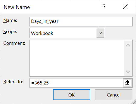
2. Type a name
3. Type your constant’s value into the Refers to box.
Excel will add an equals sign for you. Percentages will also convert to decimals, e.g. 10% = 0.1
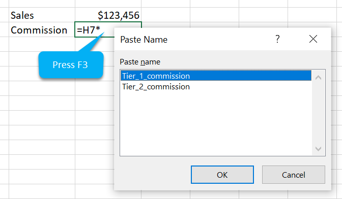
Constants are not listed in the Name Box or the Go To box but do appear in the Paste Name dialog box when you are constructing a formula.
5. How to use a named cell in a formula
When a named cell is used in a formula, the name substitutes the cell reference. There are three ways the name can be inserted into a formula.
While editing or entering the formula:
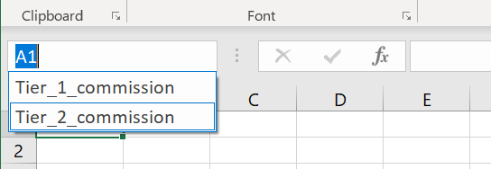
6. Using named cells for navigation
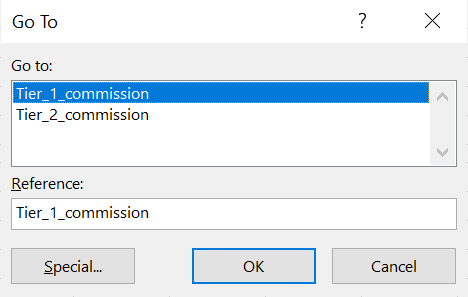
There are 2 ways to use named cell(s) to navigate to a different location in the same workbook:
TECHNIQUE 1:
1. Click the drop-down arrow on the Name Box.
2. Select a name from the list. This will take you directly to the sheet and cell.
TECHNIQUE 2:
1. Press F5 or Ctrl G to display the Go To dialog.
2. Select a name from the list.
3. Click Ok
7. Changing the cell(s) that a name refers to
To change the cell reference or cell range that a name refers to
1. Select the Name Manager icon on the Formulas ribbon.
2. Highlight the name you wish to change the details for.
3. Click the Edit button.
4. Either place the cursor in the Refers To box and carefully type your changes or delete the entire current entry and reselect from the worksheet. The second method is often easier, because when you place the cursor in the box, then use the cursor keys, a cell reference is placed in the middle of your existing entry.
5. Click Ok and then Close.
8. Removing a name from a cell
To un-name a cell (remove the name):
1. Select the Name Manager icon on the Formulas ribbon.
2. Highlight the name.
3. Click the Delete button.
9. Using table headings for naming cell ranges
To use existing column headings or row labels as the names for new named ranges:
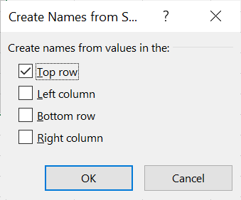
1. Select the data, including the headings.
2. Click Create from Selection on the Formulas ribbon.
3. Specify which parts of the selected range you wish to use as names. This is normally the top row or the left column or both.
4. Click Ok
10. Applying new names to existing formulas
If you have created formulas which refer to cell(s) that have since been named, you can apply the names automatically to your existing formulas.
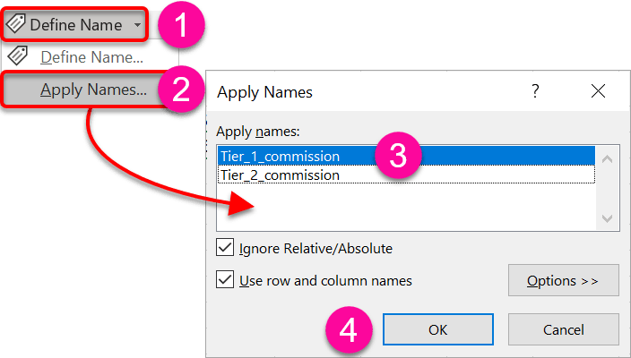
1. Select the formula cell(s) that currently refer to a cell reference or cell range that has since been named.
2. Click the drop-down arrow on the Define Name button on the Formulas ribbon.
3. Choose Apply Names. Excel selects any relevant cell names. Do not change these.
4. Click Ok
5. Check one of the original formulas and note that the name has replaced the original cell/range.
11. Displaying a summary of named cells
To display a list of named cells, ranges, constants and formulas as a printable reference:
1. Select a blank area of the worksheet where the list will be inserted.
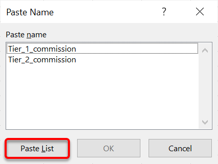
2. Click the drop-down arrow on the Use in Formula button (Formulas ribbon). The Paste Names dialog box is displayed.
3. Click Paste List. Each name is pasted onto the worksheet with its associated cell, range, constant or formula.
12. Key Takeaways
I hope you found plenty of value in this post. I'd love to hear your biggest takeaway in the comments below together with any questions you may have.
Have a fantastic day.


About the author
Jason Morrell
Jason Morrell is a professional trainer, consultant and course creator who lives on the glorious Gold Coast in Queensland, Australia.
He helps people of all levels unleash and leverage the power contained within Microsoft Office by delivering training, troubleshooting services and taking on client projects. He loves to simplify tricky concepts and provide helpful, proven, actionable advice that can be implemented for quick results.
Purely for amusement he sometimes talks about himself in the third person.
SHARE

