How to calculate the row number of the last populated cell or first populated cell in a range

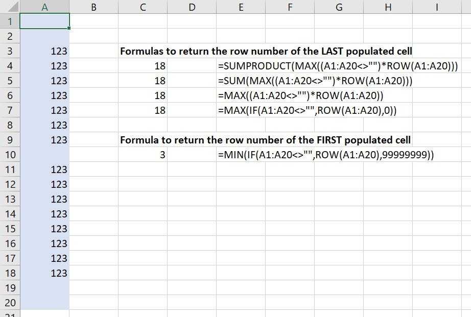
Imagine you have a range of cells where some of the cells are populated and some are empty, like those shown below.

This formula will calculate the row number of the last populated cell in the range A1:A20. That's row 18.

Modern versions of Excel are smart enough to recognise when arrays are being used. However, if you are using an older version of  Excel, or a Mac, you need to press CTRL + SHIFT + ENTER which adds braces around the entire formula and tells Excel explicitly that it is an array formula.

Caution: Don't type the braces in yourself. It won't work if you do.

Let's break this down.

An array formula is one that allows cell ranges (arrays) to be used within the formula instead of just single cell references.

SUMPRODUCT can use 1 or more arrays as long as they are the same size. It multiplies each corresponding cell of each array, then adds up the values to give a total.

Let's break the formula down.

This returns TRUE (or 1) for any cell in the range A1:A20 that is populated (I.e. not empty).

This returns the row number for each cell in the range A1:A20.

On any empty row (e.g. row 1) the test A1:A20<>"" returns FALSE or zero. Any row number multiplied by zero is zero.

On any populated row (e.g. row 3), the test A1:A20<>"" returns TRUE or 1. Any row number multiplied by 1 gives the row number.

The MAX function returns the largest result it finds in the array. In this example, that's 1 x 18 which is row 18.

In the SUMPRODUCT formula above, there is only 1 value being calculated within the SUMPRODUCT brackets - that's a single value 18 which is calculated by the MAX function.

There isn't a second array within the formula so SUMPRODUCT is overkill.

Replacing SUMPRODUCT with SUM works just as well.

As mentioned above, the MAX function returns one value - 18 - so SUM isn't required either because you are just adding up one value.

This formula works just as well.

I'm going to show you one final method. It's a slightly longer formula but it can be easily adapted to return the row number of the FIRST populated cell instead of the row number of the LAST populated cell.

Here's the formula:.

In the same way, each cell in the array A1:A20 is tested to see if it is populated. 

If it is, the row number is returned. If not, zero is returned.

In this example the resulting array is {3, 4, 5, 6, 7, 8, 9, 11, 12, 13, 14, 15, 16, 17, 18 }

The MAX function then selects the  largest number from the returned array - 18.

Adapt the formula slighly to:

You can use any number instead of 99999999 as long as it is beyond the largest number in the range.

Here is a summary of all the formulas discussed above.

You can download the example file here.

I hope you found this post useful.